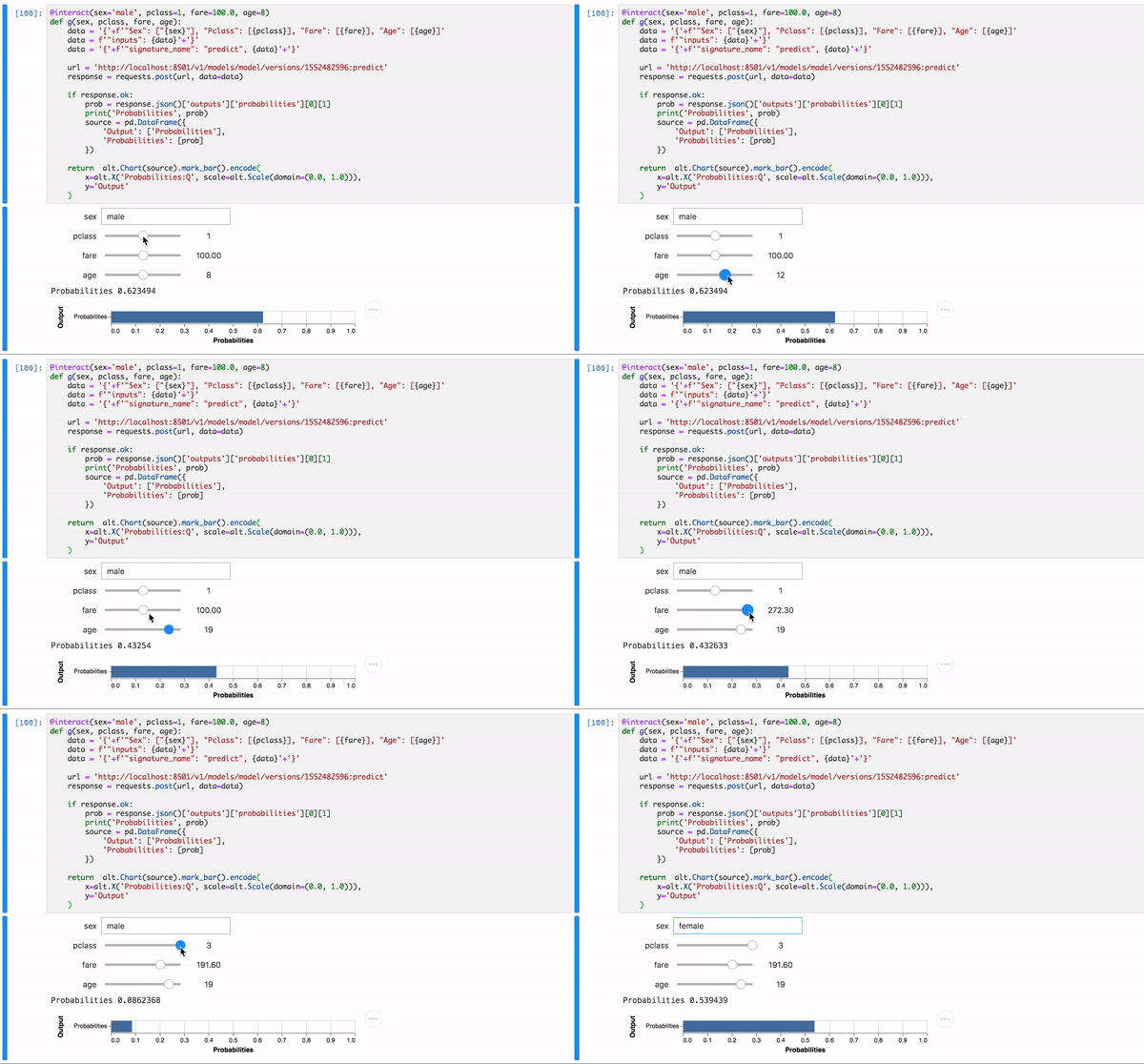
Google recently unveiled TensorFlow 2.0 developer preview at its annual summit just a couple of weeks ago, with many exciting new features and improvements introduced. Today, I’m going to walk you through how exactly to build a simple machine learning model with TF 2.0, and how to serve your model in production ready environment using TF Serving and Docker with RESTful API.
In this post, we will
- Get our data from Kaggle
- Setup dataset importing functions
- Create a feature engineering pipeline
- Train and evaluate a toy linear model
- Export the model
- Serve it with Docker via RESTful API
- Do inferencing with an interactive app
Grab some popcorns, pip install tensorflow==2.0.0-alpha0 and let’s get started.

Get our data from Kaggle
For real world public datasets, I generally turn to Kaggle, an online community of data scientists and machine learners. The Titanic datasets is freely available to benchmark ML models to predict what sorts of people were likely to survive in that historical tragic event. With Kaggle API, downloading it is a breeze:
$ kaggle competitions download -c titanic -p data
Loading them in Jupyter Notebook, we split the training data into training and validation set. We have 712, 179, 418 rows in training, validation and test samples respectively, a total of 11 features, including demographic info such as passengers’ name, gender, age and also data with respect to the voyage such as ticket class, passenger fare, etc. But for now we’re gonna skip EDA (exploratory data analysis) for the sake of time, and quickly dive into feature engineering and model training part.
TRAIN_PATH = os.path.join('data', 'train.csv')
TEST_PATH = os.path.join('data', 'test.csv')
TARGETS = 'Survived'

df = pd.read_csv(TRAIN_PATH)
df_test = pd.read_csv(TEST_PATH)
df_train, df_valid = train_test_split(df, test_size=0.2, random_state=42, shuffle=True, stratify=df[TARGETS])

df_train.shape, df_valid.shape, df_test.shape # ((712, 12), (179, 12), (418, 11))
Setup dataset importing functions
Before we jump in, we need to decide our data importing functions so can feed the data as expected when training and evaluating our model.
Note that at each stage the input function sent to the Estimator takes a different set of parameters. So we create three variants, namely train_input_fn, eval_input_fn, and lastly predict_input_fn. Each input function takes a pd.DataFrame as an argument, and outputs a tf.data.Dataset.
Create a feature engineering pipeline
Feature engineering is really at the core of how magic happens for traditional ML models. It’s basically an iterative process and has a lot of fun indeed. But since this is not the main idea of this post, things are made stupid simple. In this example, we select four features as our input columns: we can safely assume that there was a difference between Age groups as to the likelihood they could survive. Gender, or Sex also played a major role undoubtedly, which takes on either ‘male’ or ‘female’. And finally, the type of your ticket class Pclass, the price you paid for the ticket Fare.
CATEGORICAL_COLUMNS = ['Sex']
NUMERIC_COLUMNS = ['Pclass', 'Fare']
BUCKETIZED_COLUMNS = ['Age']
FEATURES_COLUMNS = CATEGORICAL_COLUMNS + NUMERIC_COLUMNS + BUCKETIZED_COLUMNS
TARGETS = 'Survived'
Feature transformations here we use are value clipping, taking log, normalization and bucketization. For example, we clip the values of Fare outside of 5 percentile on each side, and then take the log before a min-max normalization to scale them between 0 and 1.
FEATURE_CLIP_TRANS = ['Fare']
FEATURE_LOG1P_TRANS = ['Fare']
FEATURE_MIN_MAX_NORM = NUMERIC_COLUMNS
Next, we’ll get to define tf.feature_column and in the meantime implement the above feature transformation pipelines via its normalizer_fn argument.
We finally wrap the preprocessing and transformation logics all inside a norm function, which will be executed after default_value is applied. Think of that as just one of many thousand ways of doing it. Feature engineering is really something that sparks innovative ideas. The sky is your limits.
Train and evaluate a toy linear model
TensorFlow has provided several canned Estimators, which are high-level representation of complete models. They handle the details of initialization, logging, saving and restoring, and many other features. LinearClassifier is our best choice here:
linear_estimator = tf.estimator.LinearClassifier(
    feature_columns=feature_columns,
    model_dir=MODEL_DIR
)
Passing an appropriate data importing function to the instantiated Estimator, we finally kick off the training and evaluation process. Whew!
linear_estimator.train(train_input_fn)
result = linear_estimator.evaluate(eval_input_fn)
print(result)
{
    'accuracy': 0.7821229,
    'accuracy_baseline': 0.61452514,
    'auc': 0.83913046,
    'auc_precision_recall': 0.7822344,
    'average_loss': 0.47860998,
    ...
}
As for predicting on test set, all we need is a change of input function:
pred_dicts = list(linear_estimator.predict(predict_input_fn))
print(pred_dicts)
[
    {
        'logits': array([-2.2154305], dtype=float32),
        'logistic': array([0.09837335], dtype=float32),
        'probabilities': array([0.90162665, 0.09837336], dtype=float32),
        'class_ids': array([0]),
        'classes': array([b'0'], dtype=object)},
        ...
    },
]
Alright. For now, let’s assume we’ve essentially completed all necessary steps to ship a final robust model into production.
Export the model
You can export the trained model to SavedModel format, which is a standalone serialization format for Tensorflow objects, supported by TensorFlow serving as well as TensorFlow implementations other than Python.
An Estimator instance has a method dedicated to exporting models, called .export_saved_model. It requires a input function for sering, or serving_input_receiver_fn, so let’s build one, and name it serving_raw_input_fn. Since at inference time, we’ll feed raw input data instead of serialized tf.Example. This makes them easy to read for us human beings, but at expense of computing time.
Serve it with Docker via RESTful API
Everything is Dockerized nowadays. This application is not an exception.
Docker is born to be a full-fledged, lightweight tool to build isolated environment in which we can run softwares on multiple platforms in a reproducible manner. It is analogous to virtual machines (VMs), but operates in a fundamentally different way under the hood.
Building a TensorFlow docker app is a no brainer. We first pull an official TensorFlow Docker image from Docker Hub, then create and run a container instance, called tf from that image. We use -p to map our host port to the same port exposed by the container, and mount the local disk volume to the pre-specified model directory in the container so that TF-Serving will be able to load our SavedModel. Notice that here the model dir defaults to /models, whereas the model name defaults to model
$ EXPORT_BASE_DIR=/path/to/your/savedmodel/on/local/host/
$ docker pull tensorflow/serving
$ docker run -t --rm --name tf -p 8501:8501 -v "$EXPORT_BASE_DIR:/models/model" tensorflow/serving
and we’re good to go. We can request the server with data on cmd via RESTful API like below:
$ curl -d '{"signature_name":"predict","inputs":{"Sex": ["male", "female"], "Pclass": [3, 3], "Fare": [7.8292,7.0000], "Age": [34.5, 47]}}' -X POST http://localhost:8501/v1/models/model:predict
We can verify the predicted results of JSON format are the same as before.
{
    "outputs": {
        "logistic": [
            [
                0.0983734
            ],
            [
                0.469102
            ]
        ],
        "class_ids": [
            [
                0
            ],
            [
                0
            ]
        ],
        "probabilities": [
            [
                0.901627,
                0.0983734
            ],
            [
                0.530898,
                0.469102
            ]
        ],
        "classes": [
            [
                "0"
            ],
            [
                "0"
            ]
        ],
        "logits": [
            [
                -2.21543
            ],
            [
                -0.123749
            ]
        ]
    }
}
BONUS: go to http://localhost:8501/v1/models/model/, where you’ll find all SignatureDefs and input nodes that we defined in the graph previously. ![]()
Do inferencing with an interactive app
Ok, that is just good enough to be useful. We can make it visually a bit intuitive ,and hopefully, more appealing. And this is all done in lovely Python inside Notebook.
Voila!

Here’s an auxiliary Jupyter Notebook with entire working code. Fill free to check it out.